Benchmarks

We consider the problem of \(\ell_2\)-logistic regression for binary classification, or multinomial logistic regression if multiple classes are present.

Datasets

We will present the results obtained by the solvers of Cyanure on 11 datasets, presented in the Table below. The 9 first datasets can be found on the LIBSVM dataset web-page. The last two datasets were generated by encoding the MNIST and SVHN datasets with a two-layer convolutional kernel network (CKN), NIPS’16. All datasets samples are normalized with \(\ell_2\)-norm and centered for dense datasets.

Note

Many of the datasets I used are available here. Thanks to Chih-Jen for allowing me to post them here in .npz format. Note that the Criteo datasets comes from the Kaggle display advertising challenge

Dataset	Sparse	Num classes	n	p	Size (in Gb)
covtype	No	1	581012	54	0.25
alpha	No	1	500000	500	2
real-sim	No	1	72309	20958	0.044
epsilon	No	1	250000	2000	4
ocr	No	1	2500000	1155	23.1
rcv1	Yes	1	781265	47152	0.95
webspam	Yes	1	250000	16609143	14.95
kddb	Yes	1	19264097	28875157	6.9
criteo	Yes	1	45840617	999999	21
ckn_mnist	No	10	60000	2304	0.55
ckn_svhn	No	10	604388	18432	89

Setup

To select a reasonable regularization parameter \(\lambda\) for each dataset, we first split each dataset into 80% training and 20% validation, and select the optimal parameter from a logarithmic grid \(2^{-i}/n\) with \(i=1,\ldots,16\) when evaluating trained model on the validation set. Then, we keep the optimal parameter \(\lambda\), merge training and validation sets and report the objective function values in terms of CPU time for various solvers. The CPU time is reported when running the different methods on an Intel(R) Xeon(R) Gold 6130 CPU @ 2.10GHz with 128Gb of memory (in order to be able to handle the ckn_svhn dataset), limiting the maximum number of cores to 8. Note that most solvers of Cyanure are sequential algorithms that do not exploit multi-core capabilities. Those are nevertheless exploited by the Intel MKL library that we use for dense matrices. Gains with multiple cores are mostly noticeable for the methods ista, fista, and qning-ista, which are able to exploit BLAS3 (matrix-matrix multiplication) instructions. Experiments were conducted on Linux using the Anaconda Python 3.7 distribution.

In the evaluation, we include solvers that can be called from scikit-learn, such as Liblinear, LBFGS, newton-cg, or the saga implementation of scikit-learn. We run each solver with different tolerance parameter tol=0.1,0.01,0.001,0.0001 in order to obtain several points illustrating their accuracy-speed trade-off. Each method is run for at most 500 epochs.

Results

The results are presented below. There are 11 datasets, and we are going to group them into categories leading to similar conclusions. We start with those requiring a small regularization parameter (e.g., \(\lambda=1/(100n)\)), which lead to more difficult optimization problems since there is less strong convexity.

Note

I am well aware of the limitations of this study (single runs, lack of error bars) and I will try to improve it when time permits. Yet, the conclusions seem robust enough given the number of methods and datasets we used in this study.

Warning

Experiments conducted with Liblinear are obtained by using the variant shipped with scikit-learn 0.21.3, using the tolerance parameter tol=0.1. Experiments with a more recent version of liblinear will be reported soon.

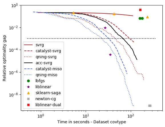
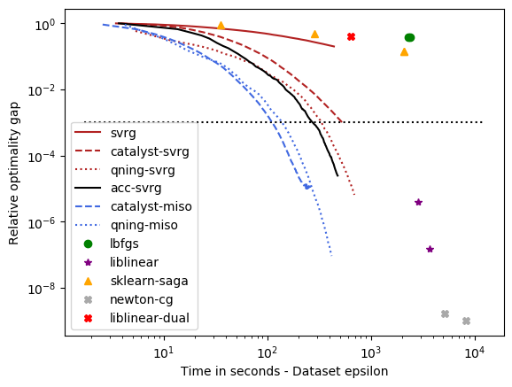
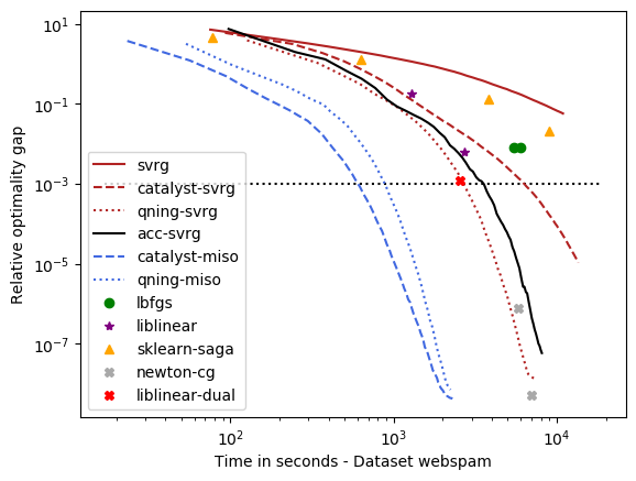
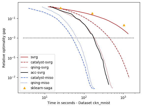
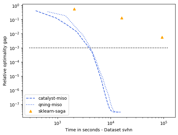
optimal \(\lambda\): covtype, epsilon, webspam, ckn_mnist, svhn – the hard ones

For these datasets, regularization is important, but not crucial to achieve a good predictive accuracy and thus the optimal \(\lambda\) is small. For instance, for ckn_mnist, the accuracy on test data is typically above 99%, and the dimension p for covtype is so small that regularization is useless. This leads to an interesting setting with clear conclusions.

Conclusions

• qning and catalyst accelerations are very useful. Note that catalyst works well in practice both for svrg and miso (regular miso, not shown on the plots, is an order of magnitude slower than its accelerated variants).

• qning-miso and catalyst-miso are the best solvers here, better than svrg variants. The main reason is the fact that for t iterations, svrg computes 3t gradients, vs. only t for the miso algorithms. miso also better handle sparse matrices (no need to code lazy update strategies, which can be painful to implement).

• Cyanure does better than sklearn-saga, lbfgs, and liblinear, sometimes with several orders of magnitudes. Note that sklearn-saga does as bad as our regular srvg solver for these dataset, which confirms that the key to obtain faster results is acceleration. Note that Liblinear-dual is very competitive on large sparse datasets (see next part of the benchmark).

• Direct acceleration (acc-svrg) works a bit better than catalyst-svrg: in fact acc-svrg is close to qning-svrg here.

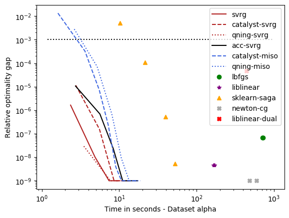
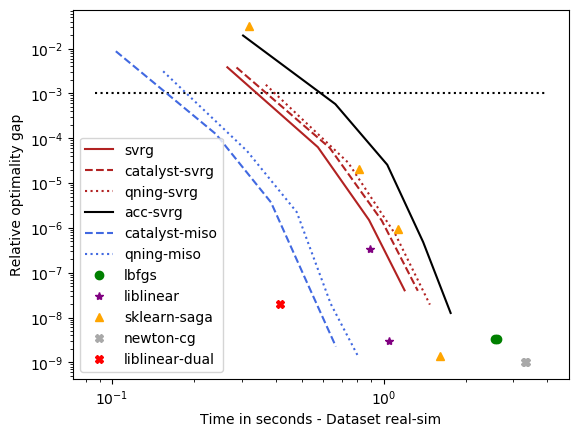
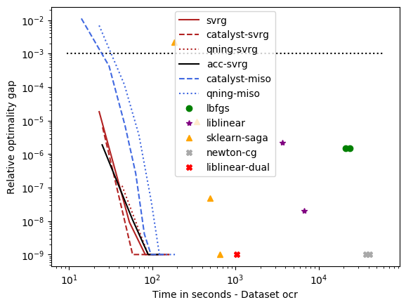
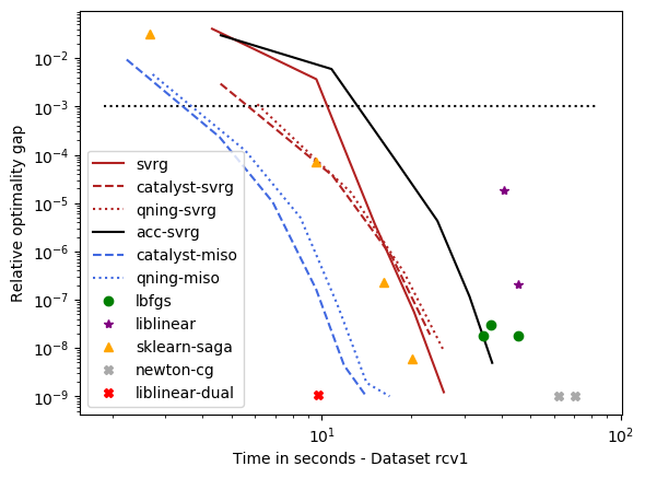
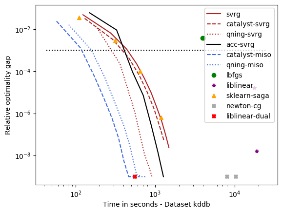
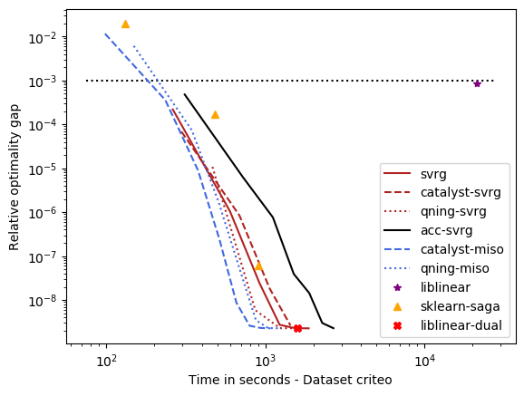
optimal \(\lambda\): alpha, rcv1, real-sim, ocr, kddb, criteo – the easy ones

For these datasets, the optimal regularization parameter is close to \(\frac{1}{n}\), which is a regime where acceleration does not bring benefits in theory. The results below are consistent with theory and we can draw the following conclusions:

• accelerations is useless here, as predicted by theory, which is why the ‘auto’ solver only uses acceleration when needed.

• qning-miso and catalyst-miso are still among the best solvers here, but the difference with svrg is smaller. sklearn-saga is sometimes competitive, sometimes not.

• Liblinear-dual is competitive on large sparse datasets.